Can we use association rules to identify co-occurring species?
Machine learning has been occupying my thoughts recently as I am reading the book Machine Learning with R by Brett Lantz (https://www.amazon.com/dp/1782162143?tag=inspiredalgor-20). I am interested in making the algorithms described in the book useful for my work in applied conservation science.
Unsurprisingly a lot of effort in machine-learning has been focused on increasing sales. One area where this has shown rapid growth is in grocery shops where loyalty cards have allowed data to be collected on our transactions. Using algorithms such as “Apriori” developed by Agrawal & Srikant in 1994, grocery shops can develop association rules which predict which products are most likely to be sold in combination. If you go to the shop and buy burgers then the chances are quite high that you will also buy burger buns to go with them. These rules allow the shops, for example, to provide offers on some products or to place certain products together on the shelves and thus encourage us to buy them more often.
Transactions are lists of products that a person has purchased. As ecologists and conservation scientists we often deal with lists of species (products) that we have observed at different sites (purchased). Can we use these association rules algorithms to identify species that are typically co-occurring? So, if we are shopping for a rare species, can we use the association rules from large datasets to predict how likely we are to find it co-occurring with other more common species.
Using the Arules R package we can mine association rules from transactions data (see this blog for an example: http://r-statistics.co/Association-Mining-With-R.html). We need some data with a lot of species from many sites to be useful for this exploration. The Natura2000 species lists contains data on over 27,000 sites in both terrestrial and marine environments. Species lists for each site are updated yearly by each European Member State. The main focus is on bird species (76% of species records are of birds), but also includes some mammals, amphibians, fish, invertebrates and plants. Clearly, this data is used here as purely an example and one should not interpret that outcomes in any ecologically meaningful way. However, ecological data are often similar in structure to these Natura2000 data.
To get the data go to https://www.eea.europa.eu/data-and-maps/data/natura-10 and download the csv file of the species data
library(arules) # allows us to mine association rules
library(arulesViz) # this is a companion package to allow more fancy visualisations from the outputs of arules
library(tidyverse) # for data manipulation
library(knitr) # for html tables
library(kableExtra)
# load the data
dat<-read.csv(choose.files(), header=TRUE, sep= ";") # this allows you to navigate to the correct folder on your own computer
# We only need the sitecode and species name columns from the data set to allow us to create "transaction" data
dat %>%
  select(SITECODE, SPECIESNAME)->dat
dat<-as.data.frame(dat)
dat<-dat[order(dat$SITECODE),]
dat<-plyr::dlply(dat,"SITECODE",c) # here we are creating a list of species for each sitecode
dat<-lapply(dat, '[[', "SPECIESNAME") # and here we are stripping out only the species list from the full list of lists above
T<-dat[-1] %>%
  head(5)

T %>%
  kable() %>%
  kable_styling()
|
|
|
|
|
For each site there is a list of species recorded in them. We can then use the Apriori algorithm to determine association using the apriori function in the arules package.
tData <- as (dat, "transactions") # we need to convert our data to a format that arules can make use of
rules <- apriori (tData, parameter = list(supp = 0.03, conf = 0.8)) # run the algorithm
## Apriori
##
## Parameter specification:
## confidence minval smax arem aval originalSupport maxtime support minlen
## 0.8 0.1 1 none FALSE TRUE 5 0.03 1
## maxlen target ext
## 10 rules FALSE
##
## Algorithmic control:
## filter tree heap memopt load sort verbose
## 0.1 TRUE TRUE FALSE TRUE 2 TRUE
##
## Absolute minimum support count: 655
##
## set item appearances ...[0 item(s)] done [0.00s].
## set transactions ...[1770 item(s), 21864 transaction(s)] done [0.08s].
## sorting and recoding items ... [173 item(s)] done [0.00s].
## creating transaction tree ... done [0.01s].
## checking subsets of size 1 2 3 4 5 done [0.04s].
## writing ... [1400 rule(s)] done [0.00s].
## creating S4 object ... done [0.00s].kable(inspect(head(rules, 3))) %>%
kable_styling()## lhs rhs support confidence
## [1] {Tetrao urogallus} => {Dryocopus martius} 0.03453165 0.8569807
## [2] {Glaucidium passerinum} => {Dryocopus martius} 0.03741310 0.9434833
## [3] {Rhinolophus euryale} => {Rhinolophus hipposideros} 0.03146725 0.8171021
## lift count
## [1] 6.206368 755
## [2] 6.832832 818
## [3] 7.250455 688| lhs | rhs | support | confidence | lift | count | ||
|---|---|---|---|---|---|---|---|
| [1] | {Tetrao urogallus} | => | {Dryocopus martius} | 0.0345317 | 0.8569807 | 6.206368 | 755 |
| [2] | {Glaucidium passerinum} | => | {Dryocopus martius} | 0.0374131 | 0.9434833 | 6.832832 | 818 |
| [3] | {Rhinolophus euryale} | => | {Rhinolophus hipposideros} | 0.0314673 | 0.8171021 | 7.250455 | 688 |
The output of the algorithm needs a little explanation. The species are listed as being on the Left-hand side (lhs) or right-hand side (rhs), so for the first rule is that Tetrao urogallus is more frequently listed with Dryocopus martius. The strength of that rule is measured in three ways. First is “support” which is calculated as the number of species lists that contains both those species divided by the total number of species lists. Confidence is the number of species lists with both species divided by the total number of species lists containing species A (in this case Tetrao urogallus). Lift is measured as the confidence divided by the expected confidence which is the number of species lists with species B (in this case Dryocopus martius) divided by the total species list. The higher the lift the more probable that the two species will occur together. The lift measure is not directional so that the rule A->B is equivalent to B->A.
So lets have a look at some of the rules and highlight the most supported
plot(rules)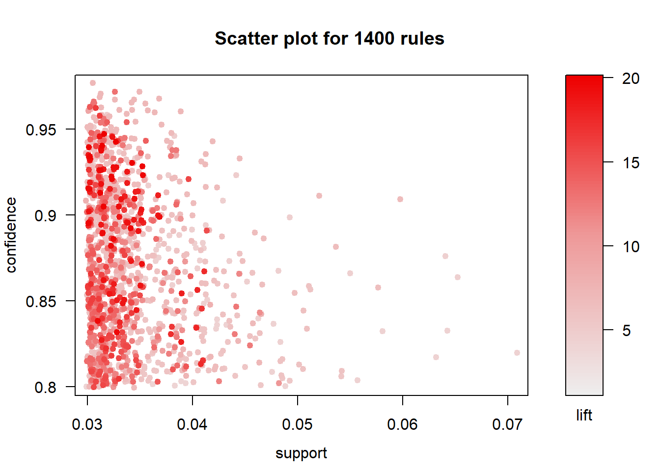
rules_conf <- sort (rules, by="confidence", decreasing=TRUE) # 'high-confidence' rules.
kable(inspect(head(rules_conf))) %>%
  kable_styling()
## lhs rhs support confidence lift count
## [1] {Botaurus stellaris,
## Philomachus pugnax,
## Tringa glareola} => {Circus aeruginosus} 0.03036956 0.9764706 7.039088 664
## [2] {Anas clypeata,
## Anas penelope,
## Anas platyrhynchos} => {Anas crecca} 0.03242774 0.9712329 12.995738 709
## [3] {Botaurus stellaris,
## Circus cyaneus} => {Circus aeruginosus} 0.03503476 0.9708492 6.998565 766
## [4] {Anas querquedula,
## Porzana porzana} => {Circus aeruginosus} 0.03119283 0.9701280 6.993366 682
## [5] {Circus cyaneus,
## Porzana porzana} => {Circus aeruginosus} 0.03100988 0.9685714 6.982145 678
## [6] {Botaurus stellaris,
## Grus grus} => {Circus aeruginosus} 0.03425723 0.9677003 6.975865 749rules_lift <- sort (rules, by="lift", decreasing=TRUE)
kable(inspect(head(rules_lift))) %>%
kable_styling() ## lhs rhs support confidence lift count
## [1] {Cuculus canorus,
## Fringilla coelebs,
## Phylloscopus collybita} => {Erithacus rubecula} 0.03160446 0.9465753 20.05419 691
## [2] {Cuculus canorus,
## Erithacus rubecula,
## Sylvia atricapilla} => {Fringilla coelebs} 0.03133004 0.9133333 20.00914 685
## [3] {Fringilla coelebs,
## Phylloscopus collybita,
## Sylvia atricapilla} => {Erithacus rubecula} 0.03261068 0.9418758 19.95463 713
## [4] {Cuculus canorus,
## Fringilla coelebs,
## Sylvia atricapilla} => {Erithacus rubecula} 0.03133004 0.9396433 19.90733 685
## [5] {Fringilla coelebs,
## Phylloscopus collybita,
## Turdus philomelos} => {Erithacus rubecula} 0.03018661 0.9388336 19.89017 660
## [6] {Cuculus canorus,
## Erithacus rubecula,
## Phylloscopus collybita} => {Fringilla coelebs} 0.03160446 0.9044503 19.81453 691##So, what do these measures of strength mean? A rule with a confidence of 1 implies that whenever we record the species on the left-hand side we also record the species on the right-hand side 100 % of the time. So for our top ranked rule for confidence when we record Botaurus stellaris, Philomachus pugnax and Tringa glareola we also record Circus aeruginosus 97% of the time.
A rule with a lift of 20 implies that, the species on the left-hand side and right-hand side are 20 times more likely to be recorded together compared to the assumption of unrelatedness.
Support is a measure of the probability that species on the left-hand side are recorded with together with those on the right-hand side in the dataset analysed.
Buying rare species
The apriori algorithm can be used to get rules for specific items. If you set the list to include only your focal species on the right-hand side you will get rules for species that it is listed with. So in our example below Turtle dove is associated with the Cyprian coal tit in 100% of the lists where the coal tit is recorded.
rules2 <- apriori (data=tData, parameter=list (supp=0.001,conf = 0.08), appearance = list (default="lhs",rhs="Streptopelia turtur"), control = list (verbose=F)) # get rules that lead to buying 'Streptopelia turtur'
rules_conf2 <- sort (rules2, by="confidence", decreasing=TRUE)
kable(inspect(head(rules_conf2))) %>%
  kable_styling()
## lhs rhs support confidence lift count
## [1] {Parus ater cypriotes} => {Streptopelia turtur} 0.00100622 1 15.23624 22
## [2] {Oenanthe cypriaca,
## Parus ater cypriotes} => {Streptopelia turtur} 0.00100622 1 15.23624 22
## [3] {Parus ater cypriotes,
## Sylvia melanothorax} => {Streptopelia turtur} 0.00100622 1 15.23624 22
## [4] {Lanius nubicus,
## Parus ater cypriotes} => {Streptopelia turtur} 0.00100622 1 15.23624 22
## [5] {Parus ater cypriotes,
## Phoenicurus ochruros} => {Streptopelia turtur} 0.00100622 1 15.23624 22
## [6] {Buteo buteo,
## Gavia arctica arctica} => {Streptopelia turtur} 0.00100622 1 15.23624 22rules3 <- apriori (data=tData, parameter=list (supp=0.001,conf = 0.15,minlen=2), appearance = list(default="rhs",lhs="Streptopelia turtur"), control = list (verbose=F)) # those who bought 'Streptopelia turtur' also bought..
rules_conf3 <- sort (rules3, by="confidence", decreasing=TRUE) # 'high-confidence' rules.
kable(inspect(head(rules_conf3))) %>%
kable_styling()## lhs rhs support confidence
## [1] {Streptopelia turtur} => {Lanius collurio} 0.04395353 0.6696864
## [2] {Streptopelia turtur} => {Hirundo rustica} 0.04029455 0.6139373
## [3] {Streptopelia turtur} => {Cuculus canorus} 0.03750457 0.5714286
## [4] {Streptopelia turtur} => {Lullula arborea} 0.03750457 0.5714286
## [5] {Streptopelia turtur} => {Caprimulgus europaeus} 0.03695573 0.5630662
## [6] {Streptopelia turtur} => {Alcedo atthis} 0.03649835 0.5560976
## lift count
## [1] 3.376072 961
## [2] 10.413596 881
## [3] 10.299847 820
## [4] 4.698651 820
## [5] 4.619467 808
## [6] 3.742234 798| lhs | rhs | support | confidence | lift | count | ||
|---|---|---|---|---|---|---|---|
| [1] | {Streptopelia turtur} | => | {Lanius collurio} | 0.0439535 | 0.6696864 | 3.376072 | 961 |
| [2] | {Streptopelia turtur} | => | {Hirundo rustica} | 0.0402945 | 0.6139373 | 10.413596 | 881 |
| [3] | {Streptopelia turtur} | => | {Cuculus canorus} | 0.0375046 | 0.5714286 | 10.299847 | 820 |
| [4] | {Streptopelia turtur} | => | {Lullula arborea} | 0.0375046 | 0.5714286 | 4.698652 | 820 |
| [5] | {Streptopelia turtur} | => | {Caprimulgus europaeus} | 0.0369557 | 0.5630662 | 4.619467 | 808 |
| [6] | {Streptopelia turtur} | => | {Alcedo atthis} | 0.0364984 | 0.5560976 | 3.742234 | 798 |
We can look at the opposite relationship by limiting the left-hand side to our focal species. Here we can see that when we record turtle dove there is a 66 % probability of recording a red-backed shrike.
##Future work We need to test this with real datasets. Can we use the association rules to give meaningful insights in to co-occurrence or at least meaningful shortcuts to survey of rare species using their associations with more common ones.
If anyone has datasets that they wish to share please feel free to get in contact.
#References
Agrawal, R., Srikant, R. 1994. Fast algorithms for mining association rules. Proceedings of the 20th International Conference on Very Large Data Bases, VLDB, pages 487-499, Santiago, Chile.
##Package citations
print(citation("arules")[2], bibtex=TRUE)##
## Hahsler M, Gruen B, Hornik K (2005). "arules - A Computational
## Environment for Mining Association Rules and Frequent Item Sets."
## _Journal of Statistical Software_, *14*(15), 1-25. ISSN 1548-7660, doi:
## 10.18637/jss.v014.i15 (URL: https://doi.org/10.18637/jss.v014.i15).
##
## A BibTeX entry for LaTeX users is
##
## @Article{,
## title = {arules -- {A} Computational Environment for Mining Association Rules and Frequent Item Sets},
## author = {Michael Hahsler and Bettina Gruen and Kurt Hornik},
## year = {2005},
## journal = {Journal of Statistical Software},
## volume = {14},
## number = {15},
## pages = {1--25},
## doi = {10.18637/jss.v014.i15},
## month = {October},
## issn = {1548-7660},
## }print(citation("arulesViz"), bibtex=TRUE)##
## Michael Hahsler (2019). arulesViz: Visualizing Association Rules and
## Frequent Itemsets. R package version 1.3-3.
## https://CRAN.R-project.org/package=arulesViz
##
## A BibTeX entry for LaTeX users is
##
## @Manual{,
## title = {arulesViz: Visualizing Association Rules and Frequent Itemsets},
## author = {Michael Hahsler},
## year = {2019},
## note = {R package version 1.3-3},
## url = {https://CRAN.R-project.org/package=arulesViz},
## }
##
## Hahsler M (2017). "arulesViz: Interactive Visualization of Association
## Rules with R." _R Journal_, *9*(2), 163-175. ISSN 2073-4859, <URL:
## https://journal.r-project.org/archive/2017/RJ-2017-047/RJ-2017-047.pdf>.
##
## A BibTeX entry for LaTeX users is
##
## @Article{,
## title = {arules{V}iz: {I}nteractive Visualization of Association Rules with {R}},
## author = {Michael Hahsler},
## year = {2017},
## journal = {R Journal},
## volume = {9},
## number = {2},
## pages = {163--175},
## url = {https://journal.r-project.org/archive/2017/RJ-2017-047/RJ-2017-047.pdf},
## month = {December},
## issn = {2073-4859},
## }print(citation("tidyverse"), bibtex=TRUE)##
## Wickham et al., (2019). Welcome to the tidyverse. Journal of Open
## Source Software, 4(43), 1686, https://doi.org/10.21105/joss.01686
##
## A BibTeX entry for LaTeX users is
##
## @Article{,
## title = {Welcome to the {tidyverse}},
## author = {Hadley Wickham and Mara Averick and Jennifer Bryan and Winston Chang and Lucy D'Agostino McGowan and Romain François and Garrett Grolemund and Alex Hayes and Lionel Henry and Jim Hester and Max Kuhn and Thomas Lin Pedersen and Evan Miller and Stephan Milton Bache and Kirill Müller and Jeroen Ooms and David Robinson and Dana Paige Seidel and Vitalie Spinu and Kohske Takahashi and Davis Vaughan and Claus Wilke and Kara Woo and Hiroaki Yutani},
## year = {2019},
## journal = {Journal of Open Source Software},
## volume = {4},
## number = {43},
## pages = {1686},
## doi = {10.21105/joss.01686},
## }print(citation("knitr")[2], bibtex=TRUE)##
## Yihui Xie (2015) Dynamic Documents with R and knitr. 2nd edition.
## Chapman and Hall/CRC. ISBN 978-1498716963
##
## A BibTeX entry for LaTeX users is
##
## @Book{,
## title = {Dynamic Documents with {R} and knitr},
## author = {Yihui Xie},
## publisher = {Chapman and Hall/CRC},
## address = {Boca Raton, Florida},
## year = {2015},
## edition = {2nd},
## note = {ISBN 978-1498716963},
## url = {https://yihui.org/knitr/},
## }print(citation("kableExtra"), bibtex=TRUE)##
## To cite package 'kableExtra' in publications use:
##
## Hao Zhu (2019). kableExtra: Construct Complex Table with 'kable' and
## Pipe Syntax. R package version 1.1.0.
## https://CRAN.R-project.org/package=kableExtra
##
## A BibTeX entry for LaTeX users is
##
## @Manual{,
## title = {kableExtra: Construct Complex Table with 'kable' and Pipe Syntax},
## author = {Hao Zhu},
## year = {2019},
## note = {R package version 1.1.0},
## url = {https://CRAN.R-project.org/package=kableExtra},
## }